5.3 SubG-CSS connection
The SubG-CSS mode allows devices to connect to the network using the ALOHA channel access protocol. The frame can be transmitted by an Endpoint when it is needed.
section 5.2.3 describes scheduling of transmission and time dependencies between downlink and uplink.
5.3.1.1 contains a detailed description of a randomization algorithm used for scheduling uplink Endpoint activities.
Each Endpoint shall communicate with the Amazon Sidewalk network to indicate its presence to the cloud and also give a Target Transmission Time to receive data. The device presence indication may be either frequent, with a specified time interval, or unscheduled, when uplink transmission is executed occasionally. Endpoints may receive data within a regulated period of time with specified intervals after uplink transmission. For more details, see section 5.5.
5.3.1 Downlink and uplink
The device working in SubG-CSS mode may start its transmission randomly. All uplink transmissions are not synchronized. The moments in time when uplink may happen are called uplink Target Transmission Times. These events are separated by a specified time interval called uplink slot separation and its value is ul_separation. Downlink shall happen after uplink transmission only. The Endpoint receive is synchronized. The moments in time when a downlink may happen are called downlink Target Transmission Times. These events are separated by a specified time interval called downlink slot separation and its value is dl_separation. Uplink transmissions are asynchronous with respect to other devices but follow a pseudo-random pattern for each device. 5.58 shows the downlink and uplink slots scheduling.
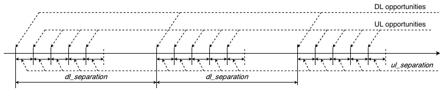
The number of uplink Target Transmission Times followed by downlink has the value nb_ul_opp.
The value nb_ul_slot has to be a power of 2
nb_ul_slot = 2 ^i where i= 0, 1, 2, …
the total amount of downlink and uplink slots nb_slot in dl_separation period is:
nb_slot = nb_ul_opp + 1
and the time consumed for all nb_slot has to be less than dl_separation time:
nb_slot \ ul_separation < dl_separation*
The number of downlink slots used for network data reception has the value nb_dl_slot. The number is counted from the last uplink transmission and the Endpoint does not schedule any further downlink when nb_dl_slot is reached. This value and dl_separation are configured by Connection Profile settings (see section 5.5).
Each uplink slot has its own index ul_slot_index in the dl_separation period and possible values are as follows:
ul_slot_index = 0, 1, ... , nb_ul_slot - 1
The method of selection of an uplink slot for a transmission is based on Lehmer’s random number generator and the result of the calculation is ul_slot_index. The index value allows calculation of the offset of an uplink slot from a downlink slot:
ul_offset = (ul_slot_index + 1) \ ul_separation*
Each uplink transmission is scheduled but not synchronized, so the time drift is not taken into account and the preamble size is constant.
5.59 shows the ul_offset and ul_opp_index values. 5.3.1.1 describes values evaluation.

fig 5.59 UL opportunity selection
Downlink slots following an uplink slot are scheduled and synchronized. The synchronization between the Endpoint and the associated Gateway is based on the uplink Epoch frame. The position in time of subsequent downlink slots is based on the uplink transmission. The Endpoint calculates ul_slot_index of the downlink slot used for transmission and ul_offset from the last downlink slot preceding the transmission. The time to the downlink slot is calculated as follows:
dl_offset = dl_separation - ul_offset
5.60 shows scheduling of downlink slots.

fig 5.60 DL opportunity estimation
An Endpoint which has been sleeping for a long time starts its transmission in case data is available to be sent. The first uplink transmission is the base for the calculation of subsequent downlink slots scheduling. Also when additional data transfer is required, the device uses scheduled downlink slots for subsequent uplink estimation. 5.61 shows such a case.

5.3.1.1 Uplink offset computation algorithm
Endpoints in close proximity can have data transmitted at a similar time. This leads to a situation where uplink activity of devices can overlap. This causes an uplink collision and a packet loss due to interference, and could happen in the case of tracking devices, for example. The uplink offset computation algorithm provides a mechanism which randomizes scheduling of uplink activities. The algorithm purpose is to calculate the ul_slot_index value which points out an uplink slot used for transmission activity.
The algorithm input for variable calculations is seed and seq_id. The seed is the table containing all UUID digits of the Endpoint and the size of the table is equal to nb_uuid of UUID digits. 5.62 shows this table.

The seq_id is the Link Layer sequence number of the Epoch frame to be transmitted (see seq_num field in Data Frame format of Link Layer in 5.1.3.2.4).
The core of the algorithm is Lehmer’s random number generator. The base equation of the generator is:
x [ n ] = ( a * x [ n - 1 ] + b ) MOD m
where n indicates the iteration number and x[n] indicates the uplink slot. Parameters m, a and b are common for all iterations. Variable m is equal to nb_ul_slot:
m = nb_ul_slot = nb_slot - 1
Variables b and a are based on the seed and calculated based on the following equations:
b = (seed[nb_uuid-1] MOD m) OR 1
a = (seed[nb_uuid-3] + (5 - (seed[nb_uuid-3] MOD 4))) MOD m;
also the initial value x[n] where n = 0 is based on seed and is calculated in the following way:
x[0] = seed[nb_uuid-2] MOD m
When UUID is changed, these three variables also need to be recalculated and the algorithm needs to be reinitialized.
The Endpoint needs to calculate a number of iterations nb_it which need to be executed for the provided seq_id. This is based on two variables curr_it and prev_it value. Variable prev_it is set to 0 during algorithm initialization:
prev_it = 0
the value curr_it is always calculated from equation
curr_it = seq_id MOD m
as this is an MOD operation; then it could happen that
curr_it < prev_it
so in this case requires recalculation of curr_it in the following way:
curr_it = (seq_id MOD m) + m
the number of iterations which needs to be executed for specified seq_id is:
nb_it = curr_it - prev_it
then the n value is increased by 1 up to nb_it in Lehmer’s equation:
n = n + nb_it
so the final x[] value for seq_id is
x[n+nb_it]
where n is the final value of all iterations executed till current seq_id. After this the prev_it is overwritten by curr_it and curr_it and is calculated again for the next seq_id.
Each new x[n] value calculated for subsequent seq_id indicates the uplink slot index ul_opp_index so ul_offset and is calculated using the following equation:
ul_offset = (ul_slot_index + 1) \ ul_separation*
This identifies the uplink slot scheduled for transmission relative to the downlink slot.